Lessons learned working with the NSIDC dataset.
Dataset: SnowEx 2021; Senator Beck Basin and Grand Mesa
Tutorial Author: Brent Wilder
Computing environment
We’ll be using the following open source Python libraries in this notebook:
from spectral import *
import numpy as np
import matplotlib.pyplot as plt
---------------------------------------------------------------------------
ModuleNotFoundError Traceback (most recent call last)
Cell In[1], line 1
----> 1 from spectral import *
2 import numpy as np
3 import matplotlib.pyplot as plt
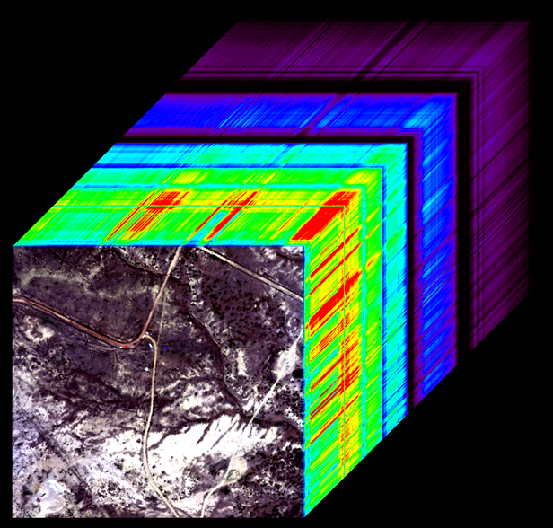
ModuleNotFoundError: No module named 'spectral'SnowEx21 Spectral Reflectance Dataset
The data were collected using an airborne imaging spectrometer, AVIRIS-NG can be downloaded from here, https://
Reflectance is provided at 5 nm spectral resolution with a range of 380-2500 nm
For this dataset, the pixel resolution is 4 m
Data span from 19 March 2021 to 29 April 2021, and were collected in two snow-covered environments in Colorado: Senator Beck Basin and Grand Mesa
Each file will have a “.img” and “.hdr”. You need to have both of these in the same directory to open data.
Downloading necessary terrain and illumination data
The NSIDC repository does not contain the terrain/illumination information.
However, you can obtain it for the matching flightline (by its timestamp) at the following URL, https://
and searching for “AVIRIS-NG L1B Calibrated Radiance, Facility Instrument Collection, V1”
You only need to download the “obs_ort” files for the flight of interest. Please note these are different than “obs” files (ort means orthorectified).
In the Granule ID search, you can use wildcars “*” on either end of “obs_ort” to reduce your search.
You may also want to use this bounding box to reduce your search:
SW: 37.55725,-108.58887
NE: 39.78206,-106.16309
Using python package, spectral, to open data
# INSERT YOUR PATHS HERE
path_to_aviris = '/data/Albedo/AVIRIS/ang20210429t191025_rfl_v2z1'
path_to_aviris_hdr = '/data/Albedo/AVIRIS/ang20210429t191025_rfl_v2z1.hdr'
path_to_terrain = '/data/Albedo/AVIRIS/ang20210429t191025_rfl_v2z1_obs_ort'
path_to_terrain_hdr = '/data/Albedo/AVIRIS/ang20210429t191025_rfl_v2z1_obs_ort.hdr'
# Open a test image
aviris = envi.open(path_to_aviris_hdr)
# Save to an array in memory
rfl_array = aviris.open_memmap(writeable=True)
# print shape. You can see here we have 425 spectral bands for a grid of 1848x699 pixels
rfl_array.shape
# You can create an array of the bands centers like this
bands = np.array(aviris.bands.centers)
bands
# A simple data visalization by selecting random indices
i = 900
j = 300
pixel = rfl_array[i,j,:]
fig, ax = plt.subplots(1, 1, figsize=(10,5))
plt.rcParams.update({'font.size': 18})
ax.scatter(bands, pixel, color='blue', s=20)
ax.set_xlabel('Wavelength [nm]')
ax.set_ylabel('Reflectance')
plt.show()Lastly, a very important note!
Please notice that convention for aspect follows to .
# Terrain bands:
# 0 - Path length (m)
# 1 - To sensor azimuth
# 2 - To sensor zenith
# 3 - To sun azimuth
# 4 - To sun zenith
# 5 - Solar phase
# 6 - Slope
# 7 - Aspect
# 8 - cosine(i) (local solar illumination angle)
# 9 - UTC Time
# 10 - Earth-sun distance (AU)

# open envi object
terrain = envi.open(path_to_terrain_hdr)

# Save to an array in memory
terrain_array = terrain.open_memmap(writeable=True)

# Grab just aspect and flatten (remove nan)
aspects = terrain_array[:,:,7].flatten()
aspects = aspects[aspects>-9999]


# Plot a histogram to show aspect range
fig, ax = plt.subplots(1, 1, figsize=(10,5))
plt.rcParams.update({'font.size': 18})
ax.hist(aspects, color='black', bins=50)
ax.set_xlabel('Aspect [degrees]')
ax.set_ylabel('Count')
plt.show()
References
To further explore these topics: