Introduction to AVIRIS-NG - Snow Observations Cookbook

Contributors:

Joachim Meyer¹, Chelsea Ackroyd¹, McKenzie Skiles¹, Phil Dennison¹, Keely Roth¹
¹University of Utah

Review of Hyperspectral Data¶

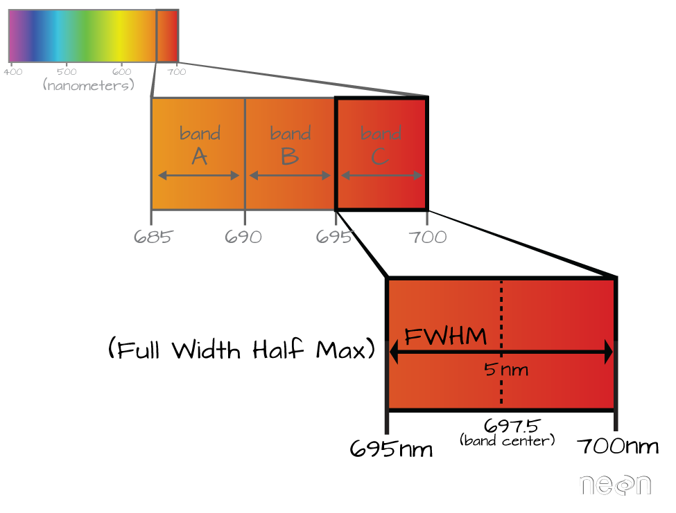
Incoming solar radiation is either reflected, absorbed, or transmitted (or a combination of all three) depending on the surface material. This spectral response allows us to identify varying surface types (e.g. vegetation, snow, water, etc.) in a remote sensing image. The spectral resolution, or the wavelength interval, determines the amount of detail recorded in the spectral response: finer spectral resolutions have bands with narrow wavelength intervals, while coarser spectral resolutions have bands with larger wavelength intervals, and therefore, less detail in the spectral response.

https://www.neonscience.org/resources/learning-hub/tutorials/hyper-spec-intro

Multispectral vs. Hyperspectral Data¶

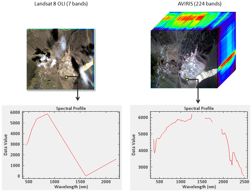
Multispectral instruments have larger spectral resolutions with fewer bands. This level of detail can be limiting in distinguishing between surface types. Hyperspectral instruments, in comparison, typically have hundreds of bands with relatively narrow wavelength intervals. The image below illustrates the difference in spectral responses between a multispectral (Landsat 8 OLI) and a hyperspectral (AVIRIS) sensor.

Computing environment¶

We’ll be using the following open source Python libraries in this notebook:

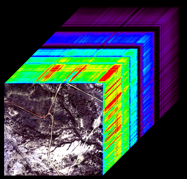
SnowEx21 Spectral Reflectance Dataset¶

The data were collected using an airborne imaging spectrometer, AVIRIS-NG can be downloaded from here, https://nsidc.org/data/snex21_ssr/versions/1.

Reflectance is provided at 5 nm spectral resolution with a range of 380-2500 nm
For this dataset, the pixel resolution is 4 m
Data span from 19 March 2021 to 29 April 2021, and were collected in two snow-covered environments in Colorado: Senator Beck Basin and Grand Mesa
Each file will have a “.img” and “.hdr”. You need to have both of these in the same directory to open data.

Accessing AVIRIS-NG Data from S3¶

For this tutorial, we’ve hosted the AVIRIS-NG data on AWS S3 for easy access. The data is streamed directly from the cloud, so no downloads are required!

The data is stored in a public S3 bucket in the us-west-2 region:

Bucket: s3://snowex-tutorials/aviris-ng/
Region: us-west-2 (Oregon)

We’ll use rasterio to read ENVI format files directly from S3. This approach:

Works with the original ENVI format (no conversion needed)
Streams data on-demand (only reads what you need)
Requires no authentication for public buckets
Enables cloud-native workflows

import rasterio
from rasterio.windows import Window
import numpy as np
import matplotlib.pyplot as plt
import os

Loading AVIRIS-NG data with rasterio¶

We’ll use rasterio to open and read the AVIRIS-NG ENVI files directly from S3.

# S3 paths for AVIRIS-NG data (public bucket, no auth required)
s3_bucket = "snowex-tutorials"
s3_prefix = "aviris-ng"
# ENVI format requires opening the .img data file (not .hdr)
reflectance_file = "SNEX21_SSR_ang20210429t191025_SBB_rfl_v2z1a_subset.img"

print(f"Data source: s3://{s3_bucket}/{s3_prefix}/{reflectance_file}")
print(f"Region: us-west-2")
print(f"\nNote: This data is publicly accessible, no AWS credentials needed!")

Data source: s3://snowex-tutorials/aviris-ng/SNEX21_SSR_ang20210429t191025_SBB_rfl_v2z1a_subset.img
Region: us-west-2

Note: This data is publicly accessible, no AWS credentials needed!

# Configure rasterio to access S3 with anonymous (no-auth) access
os.environ['AWS_NO_SIGN_REQUEST'] = 'YES'
os.environ['AWS_REGION'] = 'us-west-2'

# For ENVI files on S3, we need to use GDAL's virtual file system
vsi_path = f"/vsis3/{s3_bucket}/{s3_prefix}/{reflectance_file}"

# Open the AVIRIS-NG ENVI subset file from S3
with rasterio.Env(AWS_NO_SIGN_REQUEST='YES', AWS_REGION='us-west-2'):
    with rasterio.open(vsi_path) as src:
        print(f"Dataset dimensions: {src.width} x {src.height}")
        print(f"Number of bands: {src.count}")
        print(f"Data type: {src.dtypes[0]}")
        print(f"CRS: {src.crs}")
        print(f"\nReading reflectance data from S3...")
        print(f"  (Streaming ~21 MB - tutorial subset)")
        
        # Read all data from the subset
        rfl_array = src.read()

print(f"\nReflectance data shape: {rfl_array.shape}")
print(f"Shape interpretation: ({rfl_array.shape[0]} bands, {rfl_array.shape[1]} rows, {rfl_array.shape[2]} columns)")
print(f"\nData successfully loaded from S3!")

Dataset dimensions: 250 x 250
Number of bands: 85
Data type: float32
CRS: EPSG:32613

Reading reflectance data from S3...
  (Streaming ~21 MB - tutorial subset)


Reflectance data shape: (85, 250, 250)
Shape interpretation: (85 bands, 250 rows, 250 columns)

Data successfully loaded from S3!

# Extract wavelength information from the ENVI header metadata
vsi_path = f"/vsis3/{s3_bucket}/{s3_prefix}/{reflectance_file}"

with rasterio.Env(AWS_NO_SIGN_REQUEST='YES', AWS_REGION='us-west-2'):
    with rasterio.open(vsi_path) as src:
        # Get wavelength metadata from ENVI header
        metadata = src.tags()
        
        # ENVI headers store wavelengths as a comma-separated string
        if 'wavelength' in metadata:
            wavelength_str = metadata['wavelength'].strip('{}')
            bands = np.array([float(w.strip()) for w in wavelength_str.split(',')])
            print(f"Extracted {len(bands)} wavelength values")
            print(f"Wavelength range: {bands.min():.1f} - {bands.max():.1f} nm")
            print(f"\nFirst 10 wavelengths (nm): {bands[:10]}")
        else:
            print("Warning: Wavelength metadata not found in ENVI header")
            # Create default band indices if wavelengths aren't available
            bands = np.arange(1, rfl_array.shape[0] + 1)

Warning: Wavelength metadata not found in ENVI header

# Visualize a single pixel's spectral signature
# Note: rasterio uses (bands, rows, cols) indexing, different from (rows, cols, bands)
i = 125  # row index (middle of subset)
j = 125  # column index (middle of subset)

# Extract pixel spectrum across all bands
pixel = rfl_array[:, i, j]

fig, ax = plt.subplots(1, 1, figsize=(10,5))
plt.rcParams.update({'font.size': 18})
ax.scatter(bands, pixel, color='blue', s=20)
ax.set_xlabel('Wavelength [nm]')
ax.set_ylabel('Reflectance')
ax.set_title(f'Spectral signature at pixel ({i}, {j})')
ax.grid(True, alpha=0.3)
plt.show()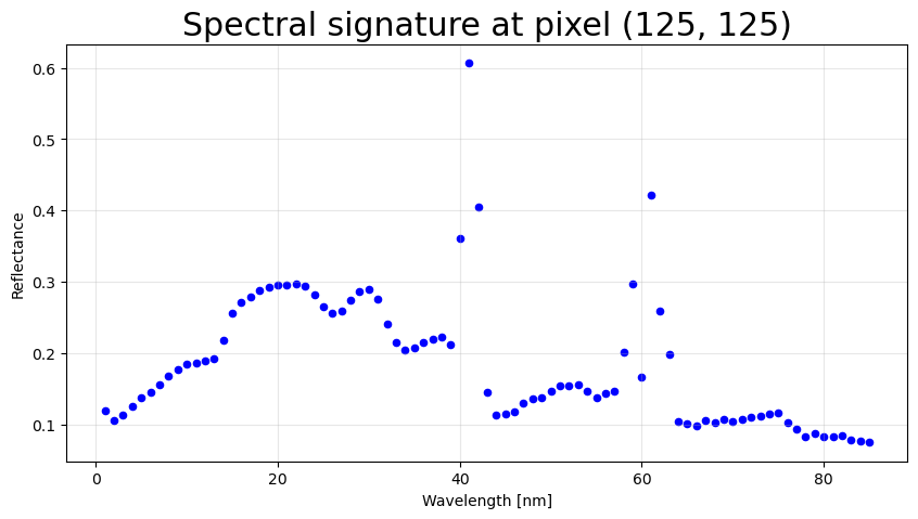

Working with Terrain Data¶

Terrain bands (when available):¶

Band 1: Path length (m)
Band 2: To sensor azimuth
Band 3: To sensor zenith
Band 4: To sun azimuth
Band 5: To sun zenith
Band 6: Solar phase
Band 7: Slope
Band 8: Aspect
Band 9: cosine(i) (local solar illumination angle)
Band 10: UTC Time
Band 11: Earth-sun distance (AU)

Important note: Aspect follows convention from $-\pi$ to $\pi$ .

Note this tutorial is incomplete. Additional content to be added from here: https://snowex-2022.hackweek.io/tutorials/aviris-ng/AVIRIS-NG_Tutorial.html